Winter Inputs Buffer Streamflow Sensitivity to Snowpack Losses in the Salt River Watershed in the Lower Colorado River Basin

Abstract

Recent streamflow declines in the Upper Colorado River Basin raise concerns about the sensitivity of water supply for 40 million people to rising temperatures. Yet, other studies in western US river basins present a paradox: streamflow has not consistently declined with warming and snow loss. A potential explanation for this lack of consistency is warming-induced production of winter runoff when potential evaporative losses are low. This mechanism is more likely in basins at lower elevations or latitudes with relatively warm winter temperatures and intermittent snowpacks. We test whether this accounts for streamflow patterns in nine gaged basins of the Salt River and its tributaries, which is a sub-basin in the Lower Colorado River Basin (LCRB). We develop a basin-scale model that separates snow and rainfall inputs and simulates snow accumulation and melt using temperature, precipitation, and relative humidity. Despite significant warming from 1968–2011 and snow loss in many of the basins, annual and seasonal streamflow did not decline. Between 25% and 50% of annual streamflow is generated in winter (NDJF) when runoff ratios are generally higher and potential evapotranspiration losses are one-third of potential losses in spring (MAMJ). Sub-annual streamflow responses to winter inputs were larger and more efficient than spring and summer responses and their frequencies and magnitudes increased in 1968–2011 compared to 1929–1967. In total, 75% of the largest winter events were associated with atmospheric rivers, which can produce large cool-season streamflow peaks. We conclude that temperature-induced snow loss in this LCRB sub-basin was moderated by enhanced winter hydrological inputs and streamflow production.

1. Introduction

The water supply of one-sixth of the world’s population is dependent upon snowmelt [1], and this reliance on snow is accentuated in dry regions like the western US, where over one-half of total runoff originates from snowmelt [2]. Reductions in snow cover and persistence across large geographic regions in recent decades [3,4,5,6] and projected shortfalls of snow storage due to climate change [2,7] suggest that streamflow loss may be widespread or imminent in many river basins. In the Upper Colorado River Basin (UCBR), which currently supplies water to 40 million people, concerns were recently heightened when warmer temperatures since the 1980s were associated with annual streamflow declines [8,9,10]. However, other studies in the western US reveal an apparent paradox: significant increases in temperatures and declines of snow storage or snowfall have not resulted in consistent streamflow losses [11,12,13,14]. Thus, temperature effects on snow and streamflow are not fully resolved and require further examination.

One possible explanation is that warming may simultaneously induce countervailing effects, reducing streamflow via one pathway, and enhancing it through another, such that individual effects are obscured, and the total effect is muted. Warmer temperatures in spring months may accelerate snow and streamflow loss due to higher rates of vapor loss to sublimation and evapotranspiration [8,15,16], and this negative feedback is likely strongest at high elevations (>3000 m) where streamflow production is heavily dependent upon snowmelt inputs. Warming has also been associated with more winter rain (less snow) [17] and earlier peak snowmelt [18]. Advancing streamflow generation to winter months could buffer spring-time losses because vapor losses are substantially lower in winter than spring months. In this case, warming would act to decouple peak water availability (winter) from peak energy demands (spring) [19] or further enhance decoupling in basins which already have distinct water and energy peaks. A recent study of snow-dominated basins in the western US demonstrated that winter runoff efficiencies are higher than spring efficiencies [20]. This phenomenon is more likely to be important in basins where winter conditions are conducive to streamflow generation, including low to mid elevations (<3000 m) with relatively warm winter temperatures and shallow snowpacks that are sensitive to small perturbations in temperature. In large mountainous river basins at lower latitudes with mixed rain and snow regimes that vary by elevation, both warming effects may occur.

Given that subsurface storage is an important precursor to streamflow, basins that experience large winter rain or snowmelt events would also be sensitive to enhanced winter streamflow under warmer conditions. A specific case is atmospheric rivers, which are large intense winter storms that typically occur under warm temperatures, resulting in higher snowlines, widespread rainfall and rain-on-snow inputs that saturate soils, and greater portions of basins that contribute to runoff. They generate 20–50% of annual streamflow in California river basins [21] and generate high runoff efficiencies and large flooding events in semi-arid Arizona [22,23]. Recent analyses along the western coast of the United States demonstrated an increase in atmospheric river activity since mid-century that may be linked to anthropogenic warming [24]. Climate models suggest that future atmospheric river activity along the US west coast will be enhanced and result in more frequent precipitation extremes and flooding events [25].

The Salt River Basin in central Arizona in the Lower Colorado River Basin (LCRB) presents an interesting case to evaluate these factors. The Salt River and its tributaries are important rivers for the regional economy, at they provide hydro-electric power and 30% of the annual water supply [26] to the sixth largest US city, Phoenix Arizona, with a population of 1.6 million. The basin has a long-term streamflow record, allowing for examination of long-term climate influences. Winters are relatively warm, snowpacks are intermittent, and individual cool-season events can have a significant impact on the timing of peak snowmelt, flooding, and annual streamflow dynamics [27,28,29]. A previous analysis in the basin found that despite significant warming in the last 50 years, annual streamflow actually increased in the last half of the 20th century after adjusting for climate variation, potentially due to greater winter rain contributions [14]. We hypothesize that warming effects in the LCRB are different than the UCRB because peak water availability and peak energy availability are more strongly decoupled temporally in the LCRB, resulting in greater runoff efficiency in winter months when evapotranspiration and sublimation losses are low [19]. Sources of fall and winter storms are quite variable, arriving from colder winter storm fronts that typically produce snowfall, but also atmospheric rivers, which often occur under warmer conditions that can produce heavy rainfall or rain-on-snow [23]. Atmospheric rivers can contribute up to 60% of cool-season precipitation totals in the Salt basin and comprise about two-thirds of the heaviest daily precipitation events (98th percentile) [22].

The goal of this study is to evaluate why warming has not caused streamflow loss in the Salt River sub-basin in the LCRB, in contrast to the documented declines in streamflow for sub-basins in the UCRB. We establish the following objectives to examine our study goal. First, we develop a basin-scale model that simulates snow accumulation and melt and separates snow and rain inputs to streamflow using temperature, precipitation, and relative humidity. Second, we use this model, streamflow data, and potential evapotranspiration (PET) estimates to examine patterns of seasonal water availability and energy demand in the Salt basins and its gaged tributaries from 1968–2011. We define three seasons based on a November–October water year as follows: winter (NDJF), spring (MAMJ), and summer-fall (JASO). In these three seasons, we evaluate magnitudes, trends, and timing of streamflow, PET, and hydrological inputs. Here, we define hydrological inputs as model estimates of snowmelt, rain-on-snow, and rainfall magnitudes that contribute to streamflow production. Third, we examine seasonal streamflow patterns at the sub-annual scale (<120 days). In part due to the influence of atmospheric rivers, which can add significant inputs to streamflow in a short amount of time, we hypothesize that streamflow responses to winter inputs would be larger and more efficient than responses in other seasons.

2. Materials and Methods

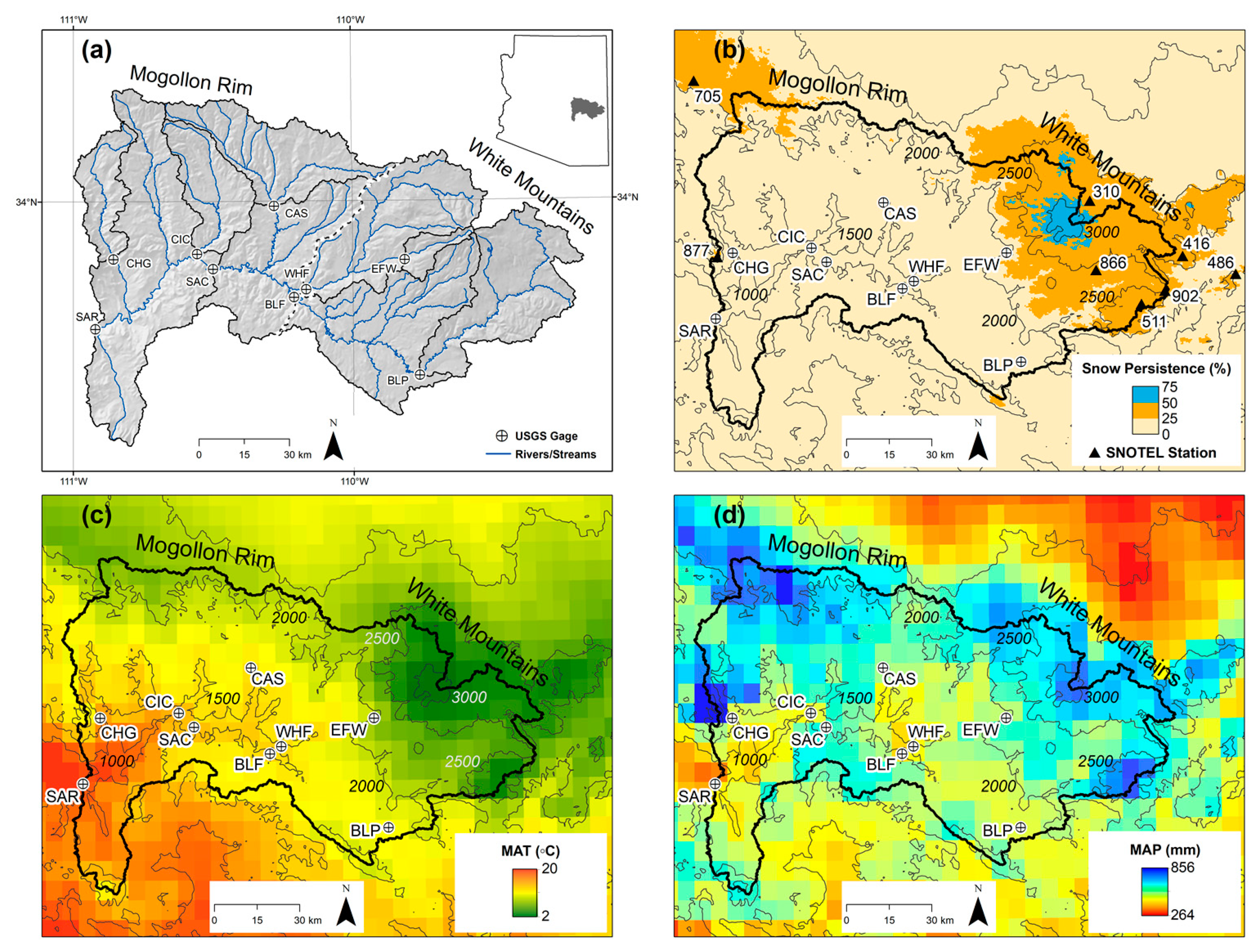
2.1. Site Description

The Salt River basin, located in northeastern Arizona south of the Mogollon Rim, covers an area of approximately 11,821 km² of mountain ranges and valleys, elevations range from 640 to 3476 meters above sea level (m.a.s.l.) (Figure 1). Vegetation changes with elevation from semi-desert scrub to ponderosa pine forest to subalpine conifer forest. Precipitation in the basin is bimodal, with frontal storms delivering snow at mid to high elevations from November to March and the North American monsoon delivering rainfall from July to September. Variability in annual precipitation is high [27,28] and dependent on heavy rainfall events, which can generate extreme flooding in the winter [22,23] and summer months [30]. Greater than 80% of the mean annual streamflow (776 million m³) occurs in winter and spring months [14]. The Salt River basin is groundwater dependent, where discharge from regional aquifers produces relatively constant baseflow (208 million m³), which is roughly one-third of the mean annual flow [31].

We examined seasonal and sub-annual hydrological patterns from 1968–2011 in nine basins within the Salt River basin above Roosevelt Dam, Arizona, USA using boundaries from the USGS Gages-II dataset [32]. For ease of presentation and conceptualization, we grouped the basins into three regions: the Salt River mainstem (2 basins), the White Mountains sub-region (4 sub-basins), and Mogollon Rim sub-region (3 sub-basins), which drain Salt mainstem tributaries on the eastern and western portions, respectively (Figure 1). To reflect the nested drainage network, Salt River mainstem gages are referred to as “basins”, and tributary gages are labeled “sub-basins” (or collectively by their sub-region). To aid comparison across basins of different sizes, all streamflow variables were normalized by basin area (i.e., specific streamflow) and expressed as depth of water (mm).

The two sub-regions differ in topographic and hydroclimatic characteristics. The White Mountains are higher in elevation and have greater snow persistence whereas the Mogollon Rim sub-basins are lower elevation and lower snow persistence (Figure 1). Mean annual precipitation in the White Mountain sub-region ranges from 550 to 653 mm [34], mean annual temperatures from 6.7–10 °C [34], and runoff ratios from 0.15–0.25 (

Table 1. Characteristics of basins within the Mogollon Rim and White Mountain sub-regions and the Salt River basin ¹.

Code	Name	USGS Gauge	Data Record	Area (km2)	Mean Elev (m)	MAT (°C)	MAP (mm)	MAQ (mm)	RR (MAQ/MAP)	Snow Persistence
White Mountains Subregion
BLP	Black River Point of Pines	9489500	1954–2011	1439	2456	6.69	637	138	0.22	34
BLF	Black River Fort Apache	9490500	1958–2011	3165	2201	8.74	549	110	0.20	32
EFW	East Fork White River	9492400	1958–2011	185	2494	10.0	597	157	0.26	38
WHF	White River Fort Apache	9494000	1958–2011	1629	2207	8.5	651	108	0.17	27
Mogollon Rim Subregion
CAS	Carrizo Creek	9496500	1953–1960, 1968–1974, 1978–2011	1142	1928	10.7	484	35	0.07	14
CHG	Cherry Creek	9497980	1966–1978, 1980–2011	517	1689	11.6	603	54	0.09	9
CIC	Cibecue Creek	9497800	1960–2009, 2011	748	1746	11.7	439	54	0.12	10
Salt River Basin
SAC	Salt River at Chrysotile	9497500	1926–2011	7327	2058	9.75	602	86	0.14	8
SAR	Salt River at Roosevelt	9498500	1916–2011	11097	1884	10.9	583	75	0.13	6

¹ MAT (mean annual temperatures) and MAP (mean annual precipitation) from 1968–2011 [34]; MAQ (mean annual streamflow) normalized by basin area; Snow persistence is percent snow persistence from 1 January–3 July from 2001–2015 [33].

). In the Mogollon Rim, mean annual temperatures are higher (10.8–11.8 °C) and mean annual precipitation (439–588 mm) and runoff ratios (0.06–0.11) lower. The Salt basin has intermediate values for all these metrics because it integrates mixed hydrological inputs and streamflow from each sub-region over a larger spatial domain. Due to greater snow accumulation and higher runoff ratios, about two-thirds of annual Salt River streamflow is generated from the White Mountains sub-region, with the remaining one-third derived from Mogollon Rim.

2.2. Data Sets

We used daily streamflow from 9 gages on the Salt River Basin above Roosevelt Dam, Arizona obtained from the USGS National Water Information System (http://waterdata.usgs.gov/nwis). Data were obtained for all basins and sub-basins from a common period, 1968–2011, and for Salt River basins from 1926–2011 (Table 1). Most of the basins had natural streamflow, unaffected by reservoirs or diversions, as indicated in the most recent USGS Annual Water Data Report (http://wdr.water.usgs.gov). Diversion records were used to compute naturalized streamflow based on withdrawals from the Black River (USGS Gage 9445000) and an addition to Carrizo Creek (USGS Gage 949500). In all basins, greater than 95% of reported daily streamflow values were classified as “observed and approved” by USGS.

As described in the next section, we developed and tested a basic snow partitioning model to evaluate sub-annual dynamics of hydrological inputs. For model development and parameter optimization, we obtained daily precipitation, temperature, and snow water equivalent (SWE) from 1993–2016 (data availability varied by station) from eight Natural Resource Conservation Service Snow Telemetry (SNOTEL) stations ranging in elevation from 2103–2781 m.a.s.l. (Figure 1,

Table 2. SNOTEL climate stations used to develop and test the snow accumulation and melt model.

Station Number	Station	Elevation (m.a.s.l.)	Water Years of Record
310	Baldy	2781	1997–2016
416	Coronado Trail	2560	1996–2016
486	Frisco Divide	2438	1993–2016
511	Hannagan Meadows	2749	1993–2016
705	Promontory	2417	1993–2016
866	Wildcat	2393	1993–2015
877	Workman Creek	2103	1993–2016
902	Beaver Head	2435	1996–2015

). We also obtained daily relative humidity for grids that overlapped each SNOTEL station from gridMET [35] because humidity is a strong control over the precipitation phase [36] and was not consistently available from station data. Before working with the SNOTEL data, we conducted a QA/QC process, which included screening for outliers and unrealistic patterns, such as flat-lined temperatures. We gap-filled missing data or data errors for temperature and SWE. If the gap was only one day of record, we filled the gap using interpolation between the days before and after the gap. For data gaps larger than one day but less than 30 days, we filled using a regression approach. For each station, we developed an equation relating the station temperature or SWE to the average of temperature and SWE from all other stations. This equation was then used to fill in the gaps. SNOTEL temperature records have an artifact caused by a shift in the sensor type. We used the approach of Ma et al. 2019 [37] to adjust the SNOTEL temperatures prior to the sensor change, so the early record temperatures would be consistent with the more recent temperature measurements.

Once model development was complete, we ran simulations of snowmelt, rain-on-snow, and rainfall inputs across the study basins for water years 1926–2011 using 6-km gridded precipitation, temperature, and relative humidity values from Livneh [34]. Before running the simulation model, we performed a QA/QC process on the forcing dataset and found unrealistic mean annual temperatures in water years 1926, 1927, 1928, and 1978; therefore, we removed these full years from the analysis. We also evaluated sub-annual patterns of energy demand, using potential evapotranspiration (PET) estimates from TerraClimate [38], which uses the Penman-Monteith method.

2.3. Snow-Rain Model

To simulate hydrologic inputs from rain, snowmelt, and rain-on-snow, we initially applied a simple temperature index snow model used in prior studies [39,40], but this produced unreliable performance across SNOTEL sites. We found that many of the largest errors were during rain-on-snow events, when snow would accumulate at a different threshold temperature than during other snow events. Therefore, we modified the model to the following:

For each day (i):

$${\mathrm{SWE}}_{\mathrm{i}}={\mathrm{SWE}}_{\mathrm{i}-1}+{\mathrm{P}}_{\mathrm{i}},\hspace{1em}\mathrm{if}\mathrm{T}\le {\mathrm{T}}_{\mathrm{s}}$$

(1)

$${\mathrm{SWE}}_{\mathrm{i}}={\mathrm{SWE}}_{\mathrm{i}-1}-{\mathsf{\alpha }\mathrm{T}}_{\mathrm{i}}-{\mathrm{P}}_{\mathrm{i}},\hspace{1em}\mathrm{if}\mathrm{T}>{\mathrm{T}}_{\mathrm{s}}$$

(2)

where SWE is the snow water equivalent in mm; P is the daily total precipitation in mm; α is the melt coefficient in mm °C⁻¹, and T_s is the daily temperature threshold in °C which varied by a relative humidity threshold (RH_t) in percent. T_s1 is the temperature threshold when humidity ≤ RH_t. T_s2 is the temperature threshold for humidity > RH_t.

In this formulation, SWE accumulates on days when precipitation and temperature are below a threshold and melts on days above the threshold using the product of temperature and a melt coefficient. Temperature thresholds vary depending on relative humidity [36]. We conducted manual calibrations of these parameters at each individual SNOTEL station to determine initial parameter values that would minimize bias. This calibration approach led to a percent bias (PBIAS) of ≤1% at all sites [41]. Next, we used the range of parameter values from the site-specific calibrations to conduct a sensitivity analysis and determine which parameters most affected SWE. The simulations performed well using the same RH_t and α, as they were most sensitive to T_s1 and T_s2.

We selected three of the parameter sets from individual site calibrations to represent low-snow, moderate-snow, and high-snow conditions (

Table 3. Model parameter values for snow water equivalent (SWE) simulations with high-snow, moderate-snow, and low-snow conditions (a) and model calibration performance statistics for daily SWE simulations (b). Calibration conducted over the SNOTEL station period of record, start dates 1993–1997 through end of water year 2016 ¹.

(a) Model Parameters
	Low Snow		Moderate Snow		High Snow
α (mm °C−1)	5.5		5.5		5.5
RHt (%)	60		60		60
Ts1 (°C)	5.5		6.8		6.8
Ts2 (°C)	2.0		2.5		3.0
(b) Model Calibration
	Low Snow		Moderate Snow		High Snow
Station	NSE	PBIAS	NSE	PBIAS	NSE	PBIAS
310	0.77	9	0.78	−1	0.74	−30
416	−0.14	92	0.32	65	0.70	21
486	0.85	6	0.79	−8	0.57	−43
511	0.89	−5	0.84	−14	0.74	−35
705	0.66	36	0.63	−42	0.45	−58
866	0.53	53	0.61	37	0.76	2
877	0.53	−7	0.47	−30	0.32	−61
902	0.80	9	0.81	−2	0.69	−29
Average	0.62	−29	0.66	1	0.61	24

¹ NSE is Nash–Sutcliffe coefficient of efficiency; PBIAS is percent bias.

a). These keep RH_t and α constant while modifying T_s values among parameter sets. To complete model calibration, we evaluated the performance of the low, moderate and high parameter sets at the SNOTEL site scale using the Nash Sutcliffe efficiency coefficient (NSE) and percent bias (PBIAS) [41]. We found that each parameter set had varying performance between stations, with the moderate snow parameter set having only 1% bias and the low and high snow parameter sets having −29% and 24% average biases, respectively (Table 3b).

Next, we conducted regional simulations with the model using forcing data for precipitation, temperature, and relative humidity from a daily 6-km dataset of Livneh [34] across the study geographic domain for water years 1926–2011. To evaluate the resulting gridded snow model output, we calculated NSE and PBIAS values of observed SWE to simulated SWE for the grids that overlapped SNOTEL stations, both at individual stations and for all stations pooled across the region. To evaluate the temporal consistency of observed to simulated SWE, we compared winter and spring trends in observed and simulated SWE using the Mann-Kendall trend test [42,43]. Trend tests were applied at individual stations and also with data aggregated across all stations using the regional Kendall test [44]. In each case, we also used the Sen Slope estimator [45] to compare magnitudes of trends.

We applied all three parameter sets (low, moderate, and high SWE) in the Livneh-forced regional gridded model to evaluate how robust our findings were to uncertainty in the snow model. To further evaluate uncertainty, we compared SWE simulations from these three versions of the regional gridded model to SWE simulations developed with the variable infiltration capacity model (VIC), which used the same forcing data [34]. While the VIC simulations were conducted over the continental United States and not calibrated individually at our study sites, we think this comparison is instructive because it compares a more physically-based model (VIC) to this study’s simpler temperature-based model using the same forcing data. Second, we compared mean monthly mean SWE estimates from this study’s gridded model to a snow gridded data set developed at the University of Arizona (termed the UA SWE dataset) [46,47], which has been shown to improve SWE estimates from prior snow models [48].

After model evaluation, we aggregated the gridded simulation output over all grid cells in each basin or sub-basin and computed:

(1)

Snowmelt (as a depth of liquid water) for days with decline in SWE;

(2)

Rain depths for days with rain but no SWE present;

(3)

Rain-on-snow depth for days with both rain and snowmelt inputs.

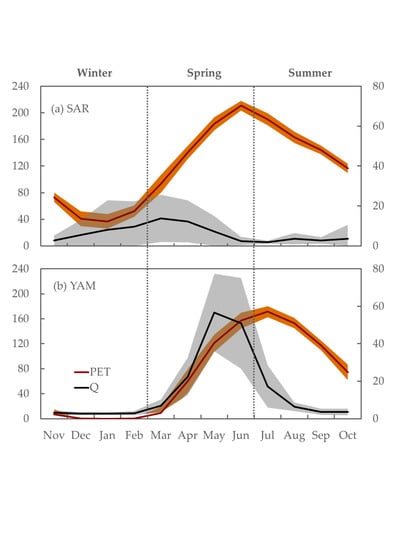
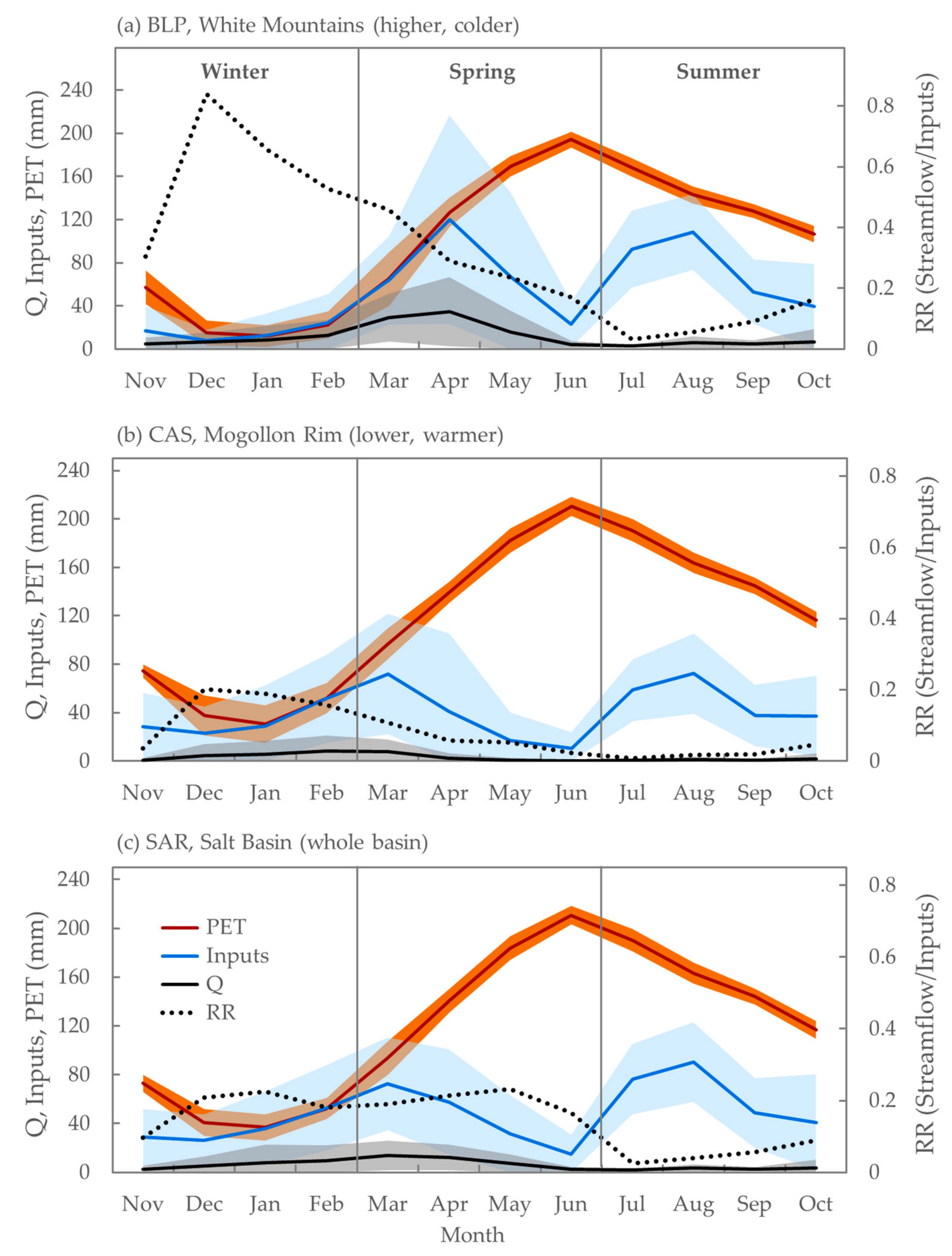
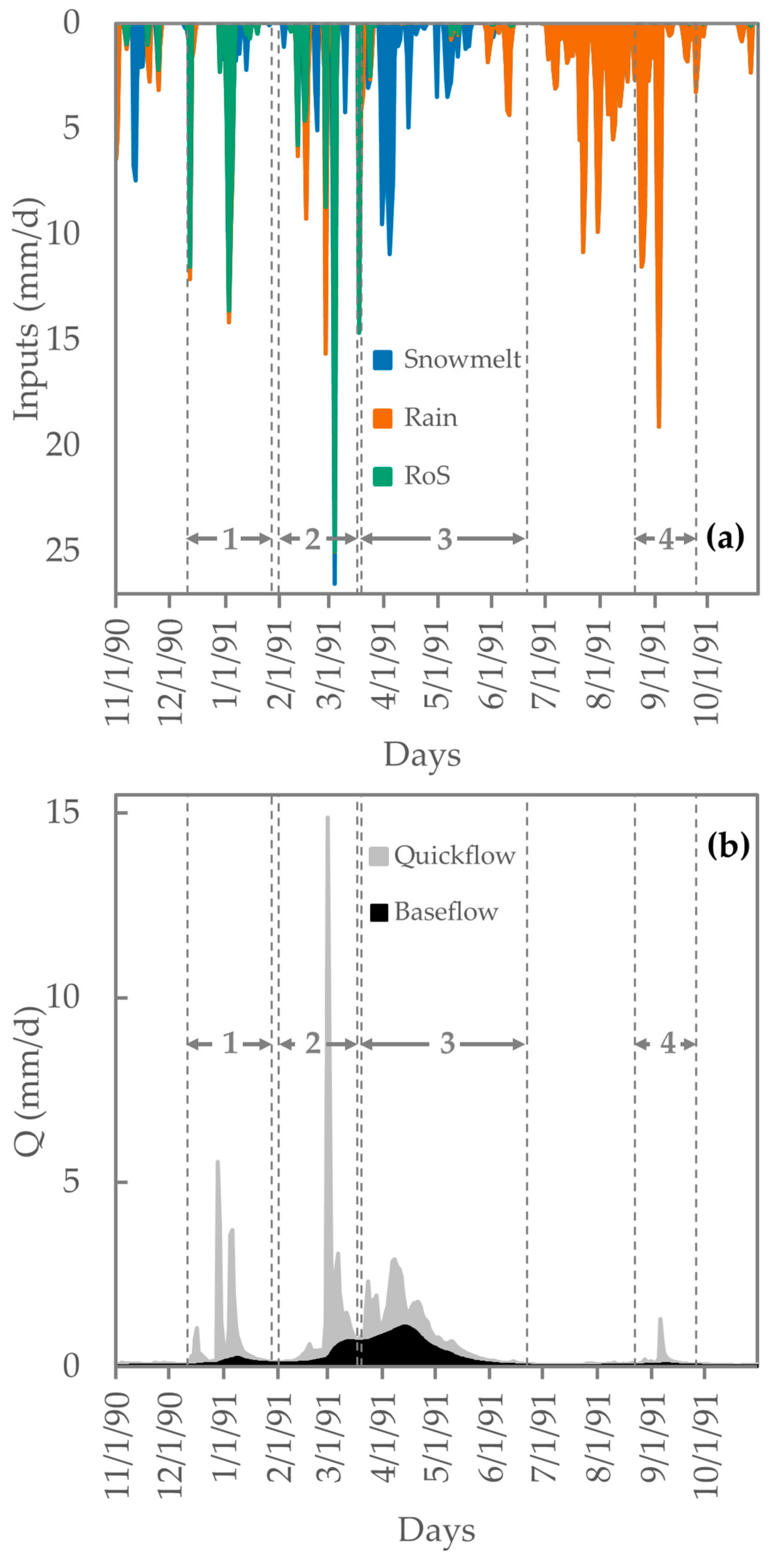
2.4. Seasonal Analyses

Using basin-scale simulations and stream gage data, we computed hydrological input and streamflow magnitudes in all the study basins in three seasons: winter (NDJF), spring (MAMJ), and summer (JASO). Seasons were calculated based upon a modified hydrologic year, November–October, that is appropriate given warm winter temperatures and a bimodal precipitation pattern. We calculated the following seasonal variables: snowmelt, rain-on-snow, rainfall, total inputs (sum on three types), area-normalized streamflow, precipitation, temperature, and PET. To standardize for variability in precipitation and temperature, we also computed fractional inputs of snowmelt, rain, and rain-on-snow in each season. Seasonal inputs, PET, and area-normalized streamflow were compared across the study’s regions, and trends and trend magnitudes were examined at the decadal scale using the Mann-Kendall test and Sen’s slope estimator, respectively.

To examine potential changes in timing, we conducted a quantile analyses on daily input and streamflow. For each day, we computed the water year cumulative input and cumulative streamflow for water years starting on 1 November. Next, we computed each day’s quantile as the fraction of water year total input or streamflow on each day and compared mean quantiles at the start of each month (e.g., 1-November, 1-December, etc.). This allowed us to evaluate differences in seasonal timing between the study basins and sub-basins. As an additional analysis, we calculated flow quantiles for each day and water year at all gauges and evaluated whether the quantiles of annual flow at the start of each month have changed over time, again using the Mann-Kendall test and Sen’s slope estimator at the decadal time scale.

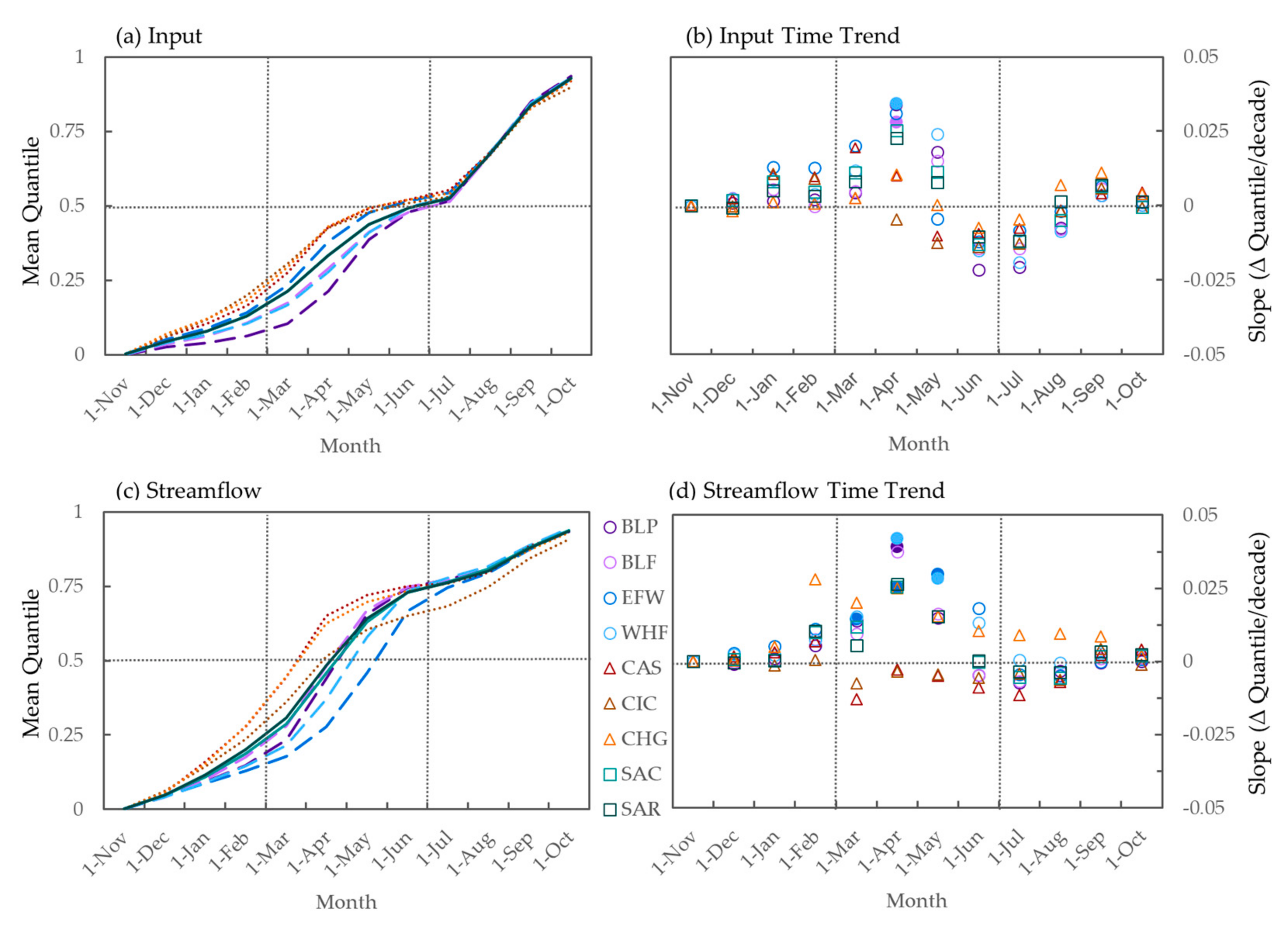
2.5. Sub-Annual Seasonal Responses

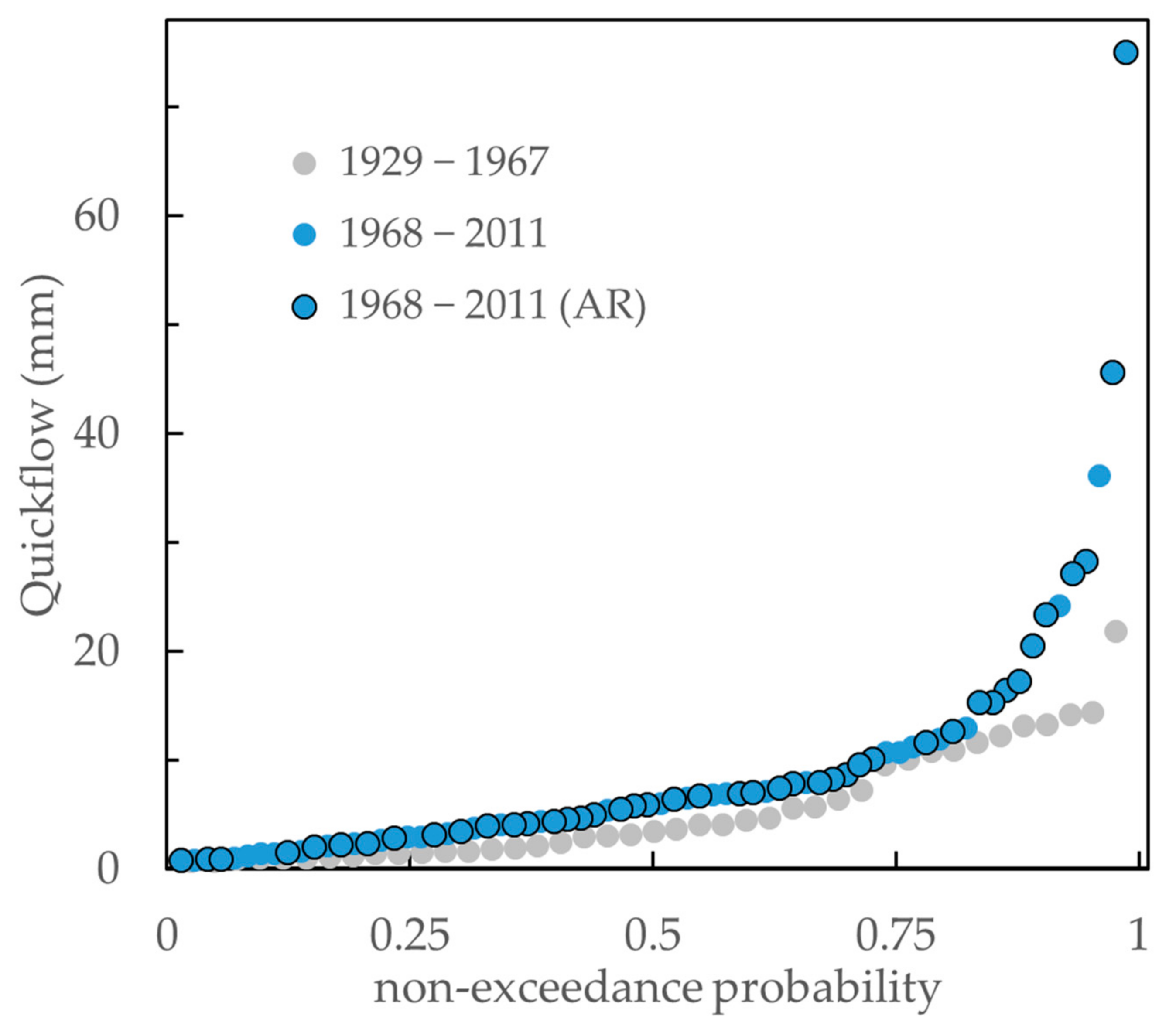
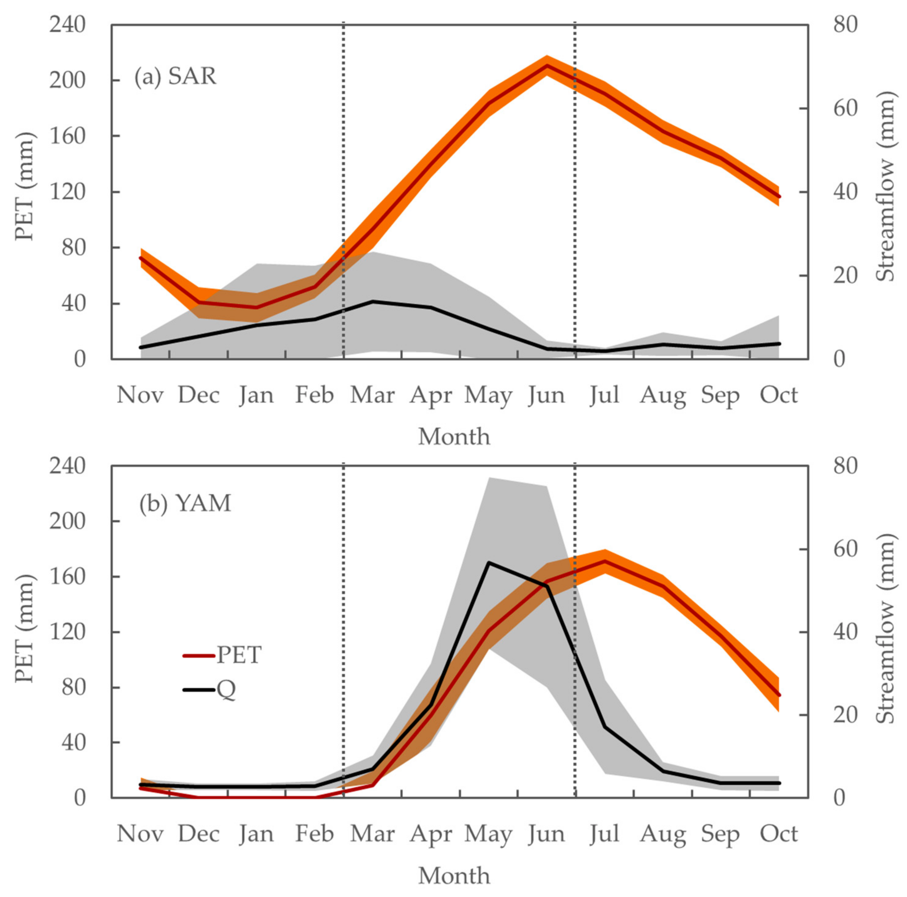
We examined whether sub-annual streamflow responses to hydrological inputs varied in different seasons of the year. Sub-annual hydrologic responses to basin inputs have durations from minutes to months depending on the input characteristics (intensity, duration, magnitude) and basin properties (antecedent storage, land cover, topography). In this study, we use the term “quickflow response intervals” (QRIs) to describe short-term streamflow responses to hydrological inputs [20]. We first separated area-normalized daily streamflow into baseflow and quickflow components using a digital filter in the Ecohydrology package in R. This filter follows the recursive digital filter method [49], which is a one-parameter signal-processing filter. We used 0.925 for the filtering parameter value following the recommendations of [50]. Then, QRIs were identified as follows: the start of a quickflow response occurred when the change in discharge (dQ/dt) was positive and this increase was >5% of the mean daily quickflow and the total quickflow increase was >10% of the mean daily quickflow. The latter two criteria were established to remove small magnitude changes in the hydrograph that were not clearly input-driven responses. The end of each response was defined, where dQ/dt was 0 or decreasing and quickflow dropped below 10% of mean daily quickflow. To ensure the analysis focused on response intervals that were relevant to annual water supply, we filtered out all QRIs where quickflow was less than 1% of mean annual streamflow of each basin. For each defined QRI, we computed duration (days), total quickflow (mm), hydrological inputs during response and 7-day prior (mm), and runoff ratio (total quickflow divided by inputs during event plus 7 days prior). To assess how QRI duration varied by season, QRIs were evaluated across 60 (1–60 days), 90 (1–90 days), and 120 (1–120 days) intervals.

QRIs were grouped by season (NDJF, MAMJ, JASO) and by study regions (White Mountains, Mogollon Rim, Salt) to increase sample size. Then, we used the Mann–Whitney U-test [51] to test for seasonal differences in quickflow magnitudes and runoff ratios (quickflow/total inputs). To evaluate whether streamflow responses had changed over time, we compared seasonal QRI magnitudes in the study period (1969–2011) to an earlier period (1929–1967) for the Salt basins. To do this, we prepared seasonal frequency distributions in these two periods and tested for differences with the Mann–Whitney U-test. Finally, we report on which QRIs overlapped with atmospheric river storms from 1979–2011 based on a previous study conducted in the Salt River Basin [22].

3. Results

3.1. Snow-Rain Model

Regional gridded snow water equivalent (SWE) simulations resulted in varying performance of simulated to observed SWE at the site versus regional scales (

Table 4. Performance statistics for gridded daily SWE simulations using high, moderate, and low snow parameter set models developed in this study for each grid cell containing a SNOTEL station and SWE simulations using Variable Infiltration Capacity (VIC) model. All simulations forced with data from [34]. Comparisons conducted over the SNOTEL station period of record, start dates 1993–1997 through end of water year 2016. Performance statistics labeled ‘Regional’ pooled all station data ¹.

Station	Low Snow		Moderate Snow		High Snow		VIC
	NSE	PBIAS	NSE	PBIAS	NSE	PBIAS	NSE	PBIAS
310	0.53	10	0.40	23	0.41	26	0.70	−24
416	0.61	21	0.36	47	0.28	58	0.76	−43
486	−3.78	158	−6.36	226	−6.61	236	0.12	−30
511	0.81	−31	0.82	−14	0.82	−8	0.64	−56
705	0.45	−59	0.62	−45	0.64	−41	0.58	−55
866	0.58	−22	0.54	9	0.47	20	0.50	−61
877	0.17	−81	0.19	−64	0.20	−64	-0.11	−98
902	0.53	−5	0.23	33	0.26	39	0.49	−63
Regional	0.54	−24	0.53	−3	0.53	2	0.57	−55

¹ NSE is Nash-Sutcliffe coefficient of efficiency; PBIAS is percent bias.

). At individual SNOTEL stations, the ‘moderate’ snow parameter set performance was very good in one, satisfactory in two, and unsatisfactory in three sites, with inconsistent results in the remaining two stations. The other parameter sets also had inconsistent performance at individual sites. Site-level simulations both underestimate SWE and overestimate SWE as shown in Figure S1. When all station data were pooled across the region, all three parameter sets had satisfactory performance, with NSE values that ranged from 0.53 to 0.54 and PBIAS values from −24 to 2. The ‘low’ parameter set under-predicted SWE (PBIAS = −24) to a greater degree than the ‘moderate’ and ‘high’ snow parameter sets. Simulated SWE using the uncalibrated VIC model had a similar performance to this study’s model for NSE (regional NSE = 0.57) but consistently underpredicted observed SWE (PBIAS −55) to a much greater degree than any of the three parameter sets. Monthly SWE from the study model had similar spatial and temporal patterns when compared to the UA SWE dataset [46,47], although the UA SWE gridded snow product also had a low snow bias, similar to VIC (not shown).

We also compared seasonal trends in observed and simulated SWE at the SNOTEL stations. Trends of simulated SWE at individual stations were generally in the same direction as observed SWE. In winter, trends in simulated SWE were in the same direction as trends in observed SWE in six of the eight stations. Trends in simulated and observed SWE in spring months were only in the same direction in three of eight sites, though the magnitudes of spring SWE trends were generally smaller than winter SWE trends. Results from the regional Kendall test, which is more resistant to outliers and missing data, showed that regional trends in simulated SWE were in the same direction and of similar magnitudes to observed SWE (Figure 2). None of the trends were significant at p < 0.05.

The performance and trend results indicate that the model simulations developed in this study have difficulty capturing complex daily and site-specific snow dynamics. However, as indicated by results when regional station data were pooled, the model simulations may be an adequate representation of SWE dynamics at the coarser spatial and temporal scales that are relevant to our study goals and objectives. Moreover, the model had less bias to observed SWE compared to other available grid snow models. Therefore, we used this model to evaluate SWE magnitudes and trends at the seasonal to sub-annual (60–120 days) temporal scales and at the regional (e.g., sub-basin to basin) spatial scale. For ease of presentation, in subsequent analyses that use the model output, we show the results from the ‘moderate’ parameter set. We also report all results from the ‘low’ and ‘high’ models in the Supplementary Materials to show the range of outcomes generated with this set of models.

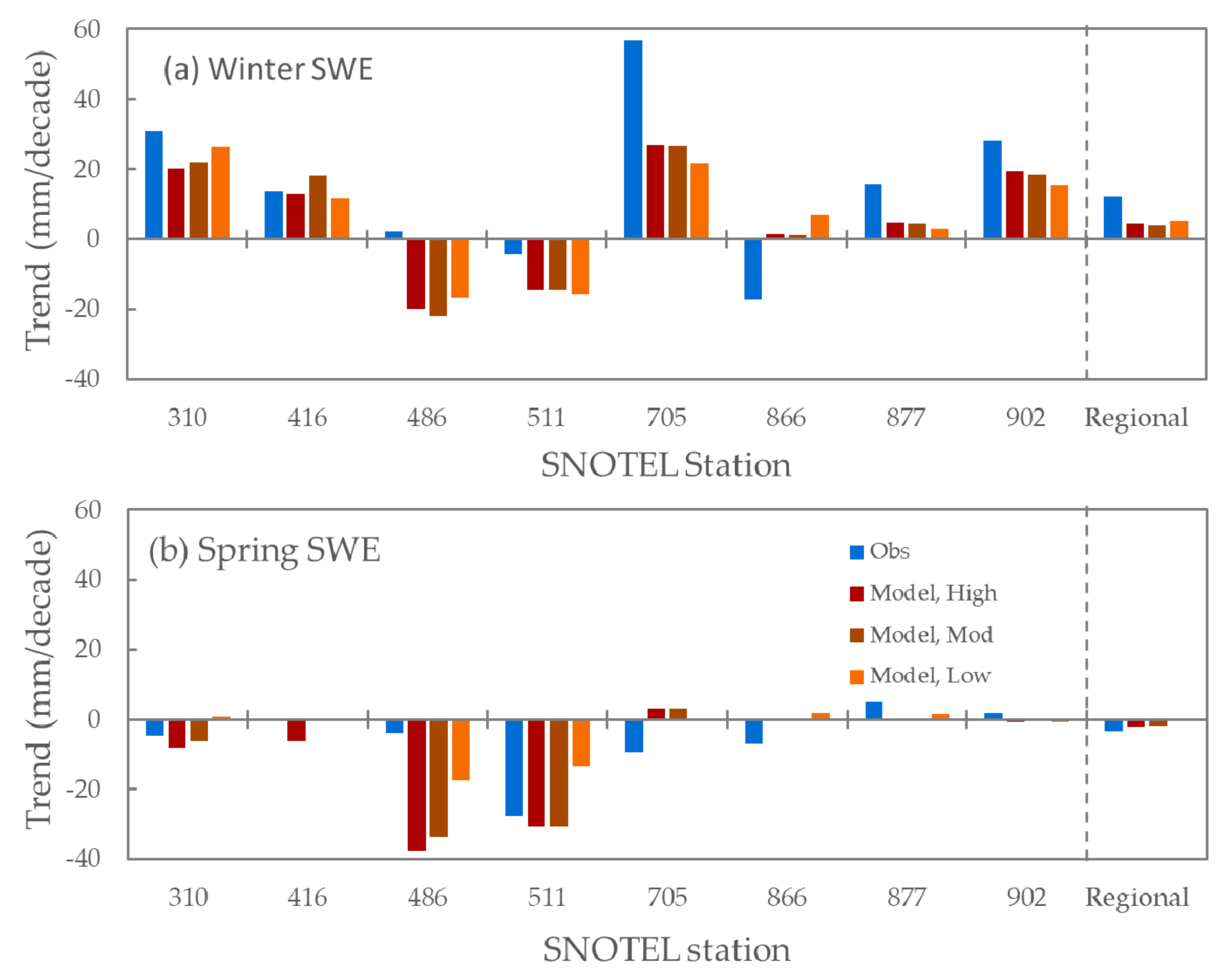
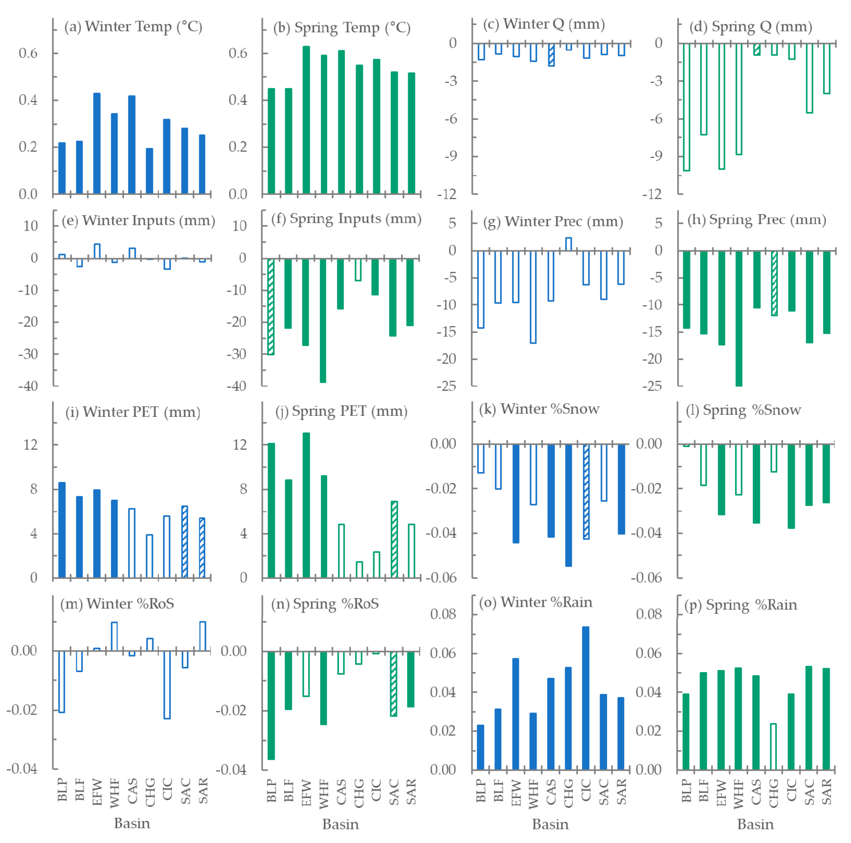
3.2. Seasonal Analyses

In the Salt River and its tributaries, greater than 80% of annual streamflow is generated in winter and spring months. One-quarter to one-half of annual production occurs in the winter season when PET rates are at annual lows (<15% of annual demand) (Figure 3). Winter streamflow production varies by sub-region, with the highest percentage in the low-elevation Mogollon Rim sub-region (mean 49%, range 41–55) and lower percentages in the White Mountains (mean 22%, range 16–31) and Salt (mean 33%, range 31–34) regions, respectively (Table S1 reports values for all sub-basins). Temperatures are warm enough that snowmelt comprised 40–50% of the winter hydrological inputs, and rain-on-snow comprised another 30–35% (Figure 3). In the ‘low snow’ model, winter snowmelt contributions are slightly lower (range 37–43%) in the Mogollon Rim and Salt regions (Table S1).

In the spring, only the high-elevation White Mountains sub-region and to a lesser extent Salt region resemble snowmelt-driven hydrographs that are typical of the Upper Colorado River Basin. The majority of annual streamflow (mean 60%, range 55–63% in White Mountains, mean 51%, range 50–53% in Salt) is produced in the spring. Spring streamflow production in the lower elevation Mogollon Rim is much lower (mean 34%, range 32–36%). Spring-time snowmelt and rain-on-snow comprise more than half of total hydrological inputs in the White Mountains and Salt regions but only 35% in the lower elevation Mogollon Rim sub-region (<30% in the ‘low snow’ model). PET demand is three times larger in spring months compared to winter months (Figure 3).

Seasonally, hydrological inputs are equal to or higher than PET in winter months, especially December and January, whereas in spring and especially summer months, PET is larger than inputs (Figure 4). Particularly in years with above-average input, winter inputs can exceed PET and result in winter-time streamflow production. Winter runoff ratios are generally higher or equal to spring ratios (Table S1). The region has a 2–4 months temporal decoupling of peak water availability, as inputs peak in March-April, whereas energy demand (PET) peaks in June. Finally, monsoon storms result in a secondary peak in hydrological inputs in summer months, but streamflow responses are muted because PET demands are several times larger than input magnitudes.

We also examined temporal trends in climate and hydrological variables from 1968–2011. Given the dominant influence of winter and spring seasons for streamflow, Figure 5 shows trends for these two seasons; trends for all metrics and seasons are reported in Table S1. Despite significant warming in winter and spring in all basins, winter and spring streamflow did not decline significantly in any basin, though trend magnitudes of spring streamflow losses were generally larger than winter losses. Additionally, springtime precipitation and hydrological inputs declined significantly in most basins, which was not the case for winter precipitation or hydrological inputs. PET increased significantly in the White Mountains region in both winter and spring, with a slightly larger increase in spring. Model simulations also suggested significant seasonal shifts in the precipitation phase, with significant increases in the percentage of hydrological inputs falling as rain (2–7% per decade) in both winter and spring and concomitant declines in percentage snowmelt (2–5% per decade) and rain-on-snow (2–4% per decade) in most basins.

Quantile trend analyses showed that input and streamflow timing varied across the study regions. The lower elevation Mogollon Rim sub-basins receive ~25% of inputs by 1-March and ~50% by 1-May (Figure 6a). In comparison, inputs in the higher elevation White Mountains region are delayed; sub-basins receive 10–20% of their inputs by 1-March and 50% by 1-June. The timing of inputs of Salt River basins is intermediate to the sub-basins as they integrate contributions from both. Streamflow generation also varies by basin elevation. The greatest streamflow generation in the Mogollon Rim region occurs 1-February to 1-April, whereas the greatest streamflow generation in the White Mountains is 1-March to 1-June (Figure 6c).

These analyses also showed trends towards earlier hydrological inputs and streamflow in spring months with subsequent declines in summer months in some basins (Figure 6b,d). Timing changes were only significant in the high-elevation White Mountains sub-region where the amount of input produced by 1-April increased (BLF, BLP, WHF). The quantiles of streamflow indicating earlier streamflow timing in winter and spring in some locations: 1-February (EFW), 1-March (EFW), 1-April (BLP, EFW, WHF), and 1-May (EFW). Note that the sub-basin with the highest mean elevation in this study, EFW, had significant changes in streamflow timing across four months, from 1-February to 1-May. Quantile estimates of the ‘moderate’ parameter set were bounded by lower and higher estimates in the ‘low’ and ‘high’ parameter sets, respectively; the trend significance of input quantiles was generally consistent across all three parameter sets (Table S2).

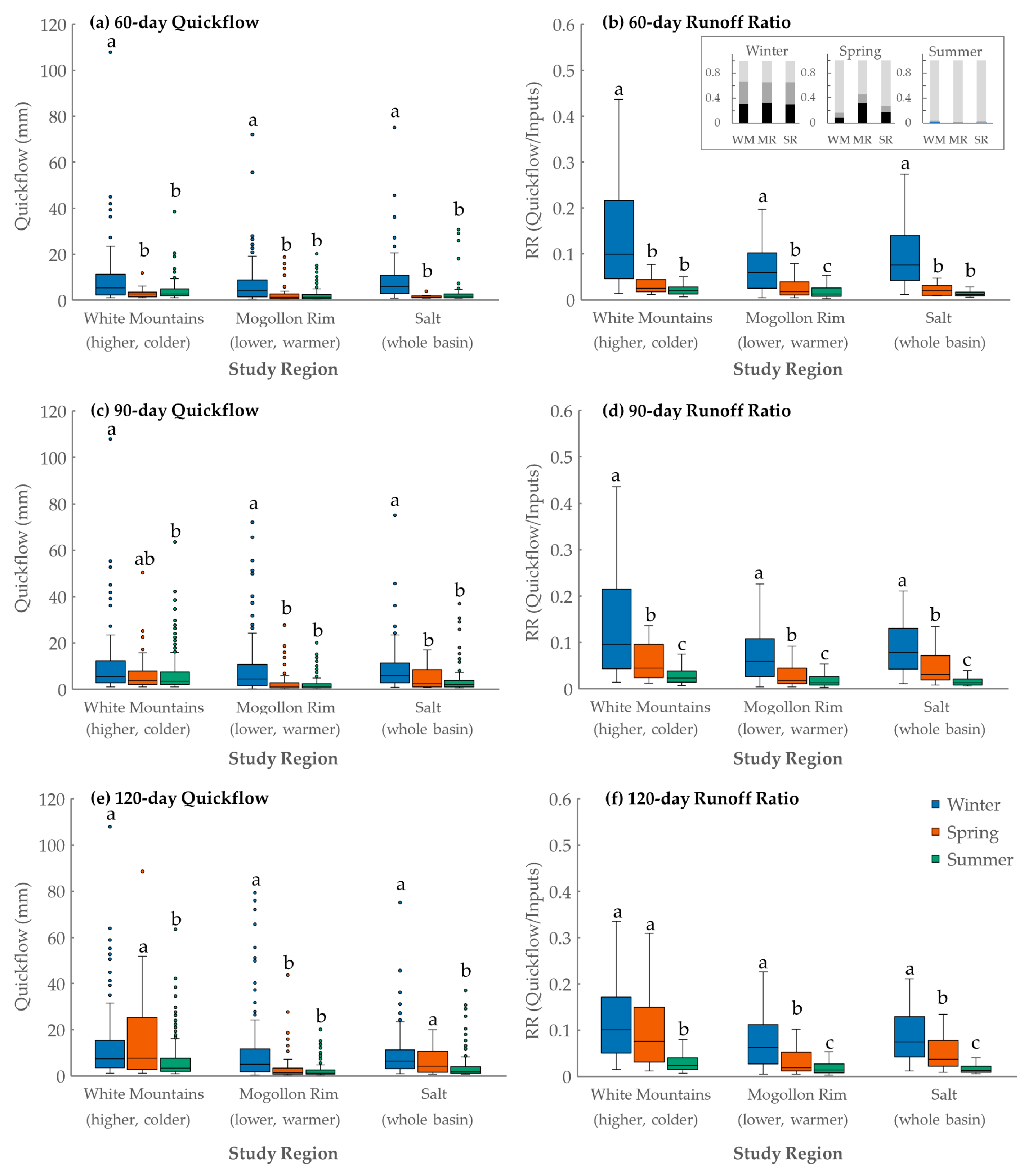
3.3. Sub-Annual Seasonal Responses

Our sub-annual analyses revealed that hydrological inputs and streamflow responses in the Salt River Basin vary throughout the year, with mixed snowmelt and rain-on-snow inputs and responses in winter, snowmelt during spring, and rainfall in summer. Figure 7 shows the timing and seasonality of these dynamics for a high-elevation sub-basin in the White Mountains, Black River near Fort Apache (BLF), in water year 1991. In this year, we identified four quickflow response intervals (QRIs), two initiated in winter, one in spring, and one in summer. The two winter QRIs occurred consecutively, the first from mid-December through January and the second starting in February and ending mid-March and both were associated with large rain-on-snow inputs. These two response intervals were likely caused by atmospheric rivers, two occurring during each response (12–13 December and 15–16 December 1990; and 28 February–1 March and 4–5 March 1991, respectively) [22]. The second interval had the 2nd largest magnitude of all QRIs identified in the BLF 1968–2011 record. The spring QRI commenced immediately after the winter responses, lasted for a longer duration, over 90 days from mid-March to late June, and exhibited a typical pattern of attenuated streamflow response from snowmelt. Despite a similar magnitude of inputs, the streamflow response of the fourth QRI in summer (August–September 1991) was of much lower magnitude, presumably due to high PET demands (Figure 3, Table S1).

Given the divergent seasonal patterns of water availability and energy demand, we explored whether seasonal QRI magnitudes and runoff ratios (quickflow/sum of inputs) varied by season. When grouped by study regions, we found that the largest quickflow magnitudes generally occurred in winter (Figure 8). At the shortest duration of 60 days, winter-time quickflow magnitudes were significantly larger than other seasons across all the study regions. Additionally, winter runoff ratios were significantly greater than other seasons across all durations (Figure 8b,d,f). The one exception was the high-elevation more snow-influenced White Mountains region where winter and spring runoff ratios at the longest duration examined (120 days) were not significantly different. Also notable was that the hydrological inputs of 60-day QRIs in winter and spring were more rain-dominated (Figure 8, inset) than seasonal means (Figure 3d–e). Across the three model parameter sets, runoff ratios were generally consistent, with the most variation in estimates occurring in the winter season in the White Mountains region (Figure S2).

Comparison of winter QRIs from an earlier period (1929–1967) to the study period (1968–2011) in the Salt River region (data not available for sub-regions) showed that short-duration (60-day) winter responses in recent decades were significantly larger than winter responses in the earlier period (Figure 9). Winter responses were nearly 2-fold larger and became more frequent in the late time period, with an average of 1.6 responses occurring every year, compared to one per year in the earlier time period. QRI magnitudes in other seasons or durations were not different in the two periods (Table S3). As shown for BLF in WY 1991, many of the high-magnitude streamflow response periods overlapped with known occurrences of atmospheric rivers. While not all atmospheric rivers were associated with high-magnitude responses, they did account for 75% of the largest winter streamflow responses (exceedance probabilities at or above 0.75) from 1979–2011 (Figure 9). The potential influence of atmospheric rivers on high-magnitude winter QRIs may be an underestimate because atmospheric river data were only available from 1979–2011.

4. Discussion

Despite significant increases in seasonal temperatures in all Salt River basins from 1968–2011 and declines in spring precipitation and hydrological inputs in most basins, streamflow magnitudes did not decline. Because more than 80% of annual streamflow is generated in winter and spring seasons, we explored whether contrasting water and energy availability dynamics in these two seasons could explain this apparent paradox. One-quarter to one-half of annual streamflow is generated in winter months, when PET demands are low (<15% of annual demand) and runoff ratios are generally higher than other seasons. Though a large portion of annual streamflow is generated in spring months (34–60%) and hydrological inputs are larger, PET demands are 3-fold greater in spring when compared to winter energy demands.

Trend and timing analyses revealed that changes in the spring season were generally larger than winter changes, though these patterns were not consistent across all basins. Increases in temperatures and decreases in hydrological inputs were larger in spring than winter months, as were declines in spring streamflow, though streamflow trends were not significant. The timing analysis showed that streamflow and hydrological inputs are occurring earlier in spring months though these trends were only significant in the higher elevation White Mountain region.

Shifting input earlier into winter can have consequences on the amount of streamflow generation. We found that magnitudes and runoff ratios of winter QRIs were generally larger than spring or summer QRIs, especially for shorter duration events (60-day) and in the lower elevation Mogollon Rim and Salt River regions. Moreover, we found that 60-day winter QRIs have increased in frequency and nearly doubled in magnitude when we compared the study period (1968–2011) to an earlier period (1929–1967) in the Salt River region (Figure 9, Table S3). Using data from a previous study [22], we found that a potential explanation for this increase is due to atmospheric rivers, which were associated with 75% of the highest magnitude 60-day winter QRIs from 1968–2011. Our simulation model also suggested that winter and spring hydrological inputs occur as rainfall, snowmelt, and rain-on-snow and that the contribution from rainfall has increased 2.5–7% per decade in both winter and spring.

Unlike recent studies that found post-1980 annual streamflow declines in the UCBR associated with rising temperatures [8,9,10], annual and seasonal streamflow did not decline in Salt River and its tributaries in this study despite monotonic warming. We note that a distinct characteristic of the Salt River and potentially LCRB sub-basins in general is a strong temporal decoupling (2–4 months) of peak water availability and energy demand. To illustrate a potential regional contrast, Figure 10 shows seasonal streamflow and PET in the Salt River (LCRB) compared to the Yampa River (UCRB). These sub-basins have been compared in previous studies because they have similar drainage areas and exhibit hydrological characteristics that are considered representative of the LCRB and UCRB, respectively [27,28]. One-quarter to one-half of streamflow is generated in the winter season in the Salt, which stands in contrast with the Yampa where the vast majority of streamflow is produced in spring and early summer months, due to later snowmelt. Moreover, peak water and energy demand overlap to a much greater degree in the Yampa compared to the Salt. This suggests that warming effects on vapor losses to sublimation and evapotranspiration are more likely to have measurable impacts on annual flow in the Yampa basin.

The higher elevation White Mountain sub-region in the Salt may be more analogous to UCBR region, but streamflow generation in April-May is still earlier [27]. In contrast to persistent snowpacks in the UCBR, LCBR snowpacks are shallow and intermittent [29] and may be more prone to producing winter runoff with small temperature fluctuations. A final regional difference is that the LCRB experiences large winter events that can produce peak flows and maximum daily flows in the winter season [22,23]. This includes atmospheric rivers, which occur under high relative humidity and warm temperatures and have produced significant winter flooding in the Salt River basin. We found that the frequency and magnitude of streamflow responses to winter inputs has increased in the last 50 years, and 75% of the largest winter responses overlapped with atmospheric rivers. Along the North American west coast, winter atmospheric river activity has increased since 1948 [24], possibly linked to increases in western Pacific sea surface temperatures that have been attributed to anthropogenic climate change [52].

The future of Salt River water provision is vital to the economy and sustainability for millions of people in the Phoenix Metropolitan Area and may be indicative of changes to other water-dependent LCRB communities. With continued warming, the counter-vailing influences that temperature has on seasonal streamflow may result in trade-offs. Our findings indicate that at the annual scale, a shift toward more winter streamflow generation may increase total streamflow. The frequency and intensity of winter flooding associated with atmospheric rivers and rain-on-snow events is projected to increase under climate change due to an intensification of extreme precipitation and more rain and less snow at higher elevations [53,54,55]. However, the combination of greater hydrologic partitioning to streamflow and earlier loss of moisture from the hillslopes implies longer, drier summers for vegetation. While the increase in winter rain and snowmelt may temporarily buffer streamflow declines from loss of snow in this region, over the long term, a shift toward all or primarily rainfall inputs in these mountains may create more dispersed input timing, which could decrease the likelihood of soil saturation and streamflow generation [56].

Annual water supply will also depend upon annual and decadal variation in hydrological inputs. Climate models project that inter-annual and decadal variability in precipitation will persist, resulting in higher streamflow in periods with above-average hydrological inputs, but also hotter and drier droughts, which could negate wet years and result in depressed baseflows in dry years [57]. The net effect of these factors on future water supply will depend upon the intensity and timing of warming, the extent and elevation of snow loss, and variation in rain and snow hydrological inputs at sub-annual to decadal scales.

We intentionally developed a simple modeling approach that could be applied using existing data sets that spanned the study period. SWE performance metrics were lower in this study than similar models at colder sites [39,40] because it was more challenging to simulate rain-snow partitioning in a warmer and more variable climate. For daily time step simulations, we found we had to use a high rain-snow temperature threshold (Table 3a) to enable snow accumulation, and this may explain why other gridded snow models [34,46,47] were biased so low for this region. We also introduced relative humidity to account for days and periods with rain-on-snow; potentially, this approach could be improved using dewpoint or wet bulb temperatures instead of relative humidity. Diurnal fluctuations in relative humidity and temperature can be quite large in this region, so simulations could potentially be improved with use of sub-daily data. Unfortunately, data at finer than daily time scales were not available across the period of record in this study. Ultimately, the modeling revealed the challenges of using standard model parameterizations in physically-based models [34,46,47] and applying simplified temperature-based snow models in this warm region. While snow model uncertainties may affect the magnitudes of estimated rain, snowmelt, and rain-on-snow inputs for each sub-basin, this should not alter our findings about the relative seasonal patterns simulated in the sub-basins and relative changes in inputs over time.

Additional factors that may have impacted our findings are forest management and our selected approach for identifying quickflow response intervals (QRIs). With respect to forest management, one recent study found that management effects on post-1960s annual streamflow in the Salt basin were negligible [14], so we expect that this would not have affected our climate-based interpretation of streamflow processes. The QRI analyses were impacted by how individual streamflow response periods were identified. Our reliance on the rising and falling limbs of quickflow may have grouped consecutive hydrograph responses if quickflow did not return to base levels between events, or may have missed rain-on-snow responses that occurred during or just prior to the snowmelt season. Given the greater frequency of large responses during wet pluvial periods, our approach may also have under-represented frequent hydrological inputs in these periods. Nonetheless, by applying the same criteria to define streamflow response periods across the time series, the relative comparisons of response periods between seasons, regions, and time periods should still be valid. As we found in this study with the use of atmospheric river data, additional analyses that compare the incidence of specific meteorological events to rain-snow partitioning and annual streamflow would add complementary information.

5. Conclusions

Historical analyses and future projections that warming is primarily a driver of streamflow loss in the Colorado River Basin likely paint an incomplete picture, particularly in basins with substantial winter streamflow generation, intermittent snowpacks, and large winter meteorological events. Here, we showed that the Salt River basin is warm enough to generate winter streamflow, which makes it somewhat resilient to temperature-related snow loss because streamflow production and efficiencies are high in winter months when energy-driven evaporative losses are low. The buffering of snow loss with winter inputs is likely to be time limited and elevation dependent because additional snow loss may eventually create a hydrologic regime to be more dispersed and rainfall dominated. When gages are nested within large river basins, future studies that examine input and streamflow dynamics in lower elevation sub-basins could help forecast imminent changes in higher elevation sub-basins. Additionally, the buffering of snow loss with winter inputs that is now apparent in the warmer southwest US could be a harbinger of future changes in colder and higher elevation basins in the western US. Such studies could help water managers develop strategies to anticipate and respond to future climate change effects.

References

1. Barnett, T.P.; Adam, J.C.; Lettenmaier, D.P. Potential impacts of a warming climate on water availability in snow-dominated regions. Nature 2005, 438, 303–309. [Google Scholar] [CrossRef]
2. Li, D.; Wrzesien, M.L.; Durand, M.; Adam, J.; Lettenmaier, D.P. How much runoff originates as snow in the western United States, and how will that change in the future? Western U.S. Snowmelt-Derived Runoff. Geophys. Res. Lett. 2017, 44, 6163–6172. [Google Scholar] [CrossRef] [Green Version]
3. Hammond, J.C.; Saavedra, F.A.; Kampf, S.K. Global snow zone maps and trends in snow persistence 2001–2016. Int. J. Clim. 2018, 38, 4369–4383. [Google Scholar] [CrossRef]
4. Kim, Y.; Kimball, J.S.; Robinson, D.A.; Derksen, C. New satellite climate data records indicate strong coupling between recent frozen season changes and snow cover over high northern latitudes. Environ. Res. Lett. 2015, 10, 084004. [Google Scholar] [CrossRef] [Green Version]
5. Mote, P.W.; Li, S.; Lettenmaier, D.P.; Xiao, M.; Engel, R. Dramatic declines in snowpack in the western US. Npj Clim. Atmos. Sci. 2018, 1, 2. [Google Scholar] [CrossRef]
6. Xu, W.; Ma, L.; Ma, M.; Zhang, H.; Yuan, W. Spatial–Temporal Variability of Snow Cover and Depth in the Qinghai–Tibetan Plateau. J. Clim. 2017, 30, 1521–1533. [Google Scholar] [CrossRef]
7. McCabe, G.J.; Wolock, D.M. Warming may create substantial water supply shortages in the Colorado River basin. Geophys. Res. Lett. 2007, 34, 5. [Google Scholar] [CrossRef] [Green Version]
8. McCabe, G.J.; Wolock, D.M.; Pederson, G.T.; Woodhouse, C.A.; McAfee, S. Evidence that Recent Warming Is Reducing Upper Colorado River Flows. Earth Interact. 2017, 21, 1–14. [Google Scholar] [CrossRef] [Green Version]
9. Udall, B.; Overpeck, J. The twenty-first century Colorado River hot drought and implications for the future. Water Resour. Res. 2017, 53, 2404–2418. [Google Scholar] [CrossRef] [Green Version]
10. Woodhouse, C.A.; Pederson, G.T.; Morino, K.; McAfee, S.A.; McCabe, G.J. Increasing influence of air temperature on upper Colorado River streamflow. Geophys. Res. Lett. 2016, 432, 174–2181. [Google Scholar] [CrossRef] [Green Version]
11. Chavarria, S.B.; Gutzler, D.S. Observed Changes in Climate and Streamflow in the Upper Rio Grande Basin. JAWRA J. Am. Water Resour. Assoc. 2018, 54, 644–659. [Google Scholar] [CrossRef] [Green Version]
12. McCabe, G.J.; Wolock, D.M.; Valentin, M. Warming is Driving Decreases in Snow Fractions While Runoff Efficiency Remains Mostly Unchanged in Snow-Covered Areas of the Western United States. J. Hydrometeorol. 2018, 19, 803–814. [Google Scholar] [CrossRef]
13. Nayak, A.; Marks, D.; Chandler, D.G.; Seyfried, M. Long-term snow, climate, and streamflow trends at the Reynolds Creek Experimental Watershed, Owyhee Mountains, Idaho, United States. Water Resour. Res. 2010, 46, W06519. [Google Scholar] [CrossRef]
14. Robles, M.D.; Turner, D.S.; Haney, J.A. A century of changing flows: Forest management changed flow magnitudes and warming advanced the timing of flow in a southwestern US river. PLoS ONE 2017, 12, e0187875. [Google Scholar] [CrossRef] [PubMed] [Green Version]
15. Christensen, N.S.; Lettenmaier, D.P. A multimodal ensemble approach to assessment of climate change impacts on the hydrology and water resources of the Colorado River Basin. Hydrol. Earth Syst. Sci. 2007, 11, 1417–1434. [Google Scholar] [CrossRef] [Green Version]
16. Molotch, N.P.; Brooks, P.D.; Burns, S.P.; Litvak, M.; Monson, R.K.; McConnell, J.R.; Musselman, K. Ecohydrological controls on snowmelt partitioning in mixed-conifer sub-alpine forests. Ecohydrol. 2009, 2, 129–142. [Google Scholar] [CrossRef]
17. Knowles, N.; Dettinger, M.D.; Cayan, D.R. Trends in snowfall versus rainfall in the Western United States. J. Clim. 2006, 19, 4545–4559. [Google Scholar] [CrossRef] [Green Version]
18. Stewart, I.T.; Cayan, D.R.; Dettinger, M.D. Changes toward earlier streamflow timing across Western North America. J. Clim. 2005, 18, 1136–1155. [Google Scholar] [CrossRef]
19. Jeton, A.E.; Dettinger, M.D.; Smith, J.L. Potential Effects of Climate Change on Streamflow, Eastern and Western Slopes of the Sierra Nevada, California and Nevada. U.S. Geological Survey Water Resources Investigations Report 95-4260; 1996. Available online: https://pubs.usgs.gov/wri/1995/4260/report.pdf (accessed on 21 December 2020).
20. Hammond, J.C.; Kampf, S.K. Subannual Streamflow Responses to Rainfall and Snowmelt Inputs in Snow-Dominated Watersheds of the Western United States. Water Resour. Res. 2020, 56. [Google Scholar] [CrossRef]
21. Dettinger, M.D.; Ralph, F.M.; Das, T.; Neiman, P.J.; Cayan, D.R. Atmospheric Rivers, Floods and the Water Resources of California. Water 2011, 3, 445–478. [Google Scholar] [CrossRef]
22. Demaria, E.M.C.; Dominguez, F.; Hu, H.; von Glinski, G.; Robles, M.; Skindlov, J.; Walter, J. Observed Hydrologic Impacts of Landfalling Atmospheric Rivers in the Salt and Verde River Basins of Arizona, United States. Water Resour. Res. 2017, 53, 10025–10042. [Google Scholar] [CrossRef]
23. Neiman, P.J.; Ralph, F.M.; Moore, B.J.; Hughes, M.; Mahoney, K.M.; Cordeira, J.M.; Dettinger, M.D. The landfall and inland penetration of a flood-producing atmospheric river in Arizona. Part I: Observed synoptic-scale, orographic, and hydrometeorological characteristics. J. Hydrometeorol. 2013, 14, 460–484. [Google Scholar] [CrossRef]
24. Gershunov, A.; Shulgina, T.; Ralph, F.M.; Lavers, D.A.; Rutz, J.J. Assessing the climate-scale variability of atmospheric rivers affecting western North America: Atmospheric River Climate-Scale Behavior. Geophys. Res. Lett. 2017, 44, 7900–7908. [Google Scholar] [CrossRef]
25. Payne, A.E.; Demory, M.-E.; Leung, L.R.; Ramos, A.M.; Shields, C.A.; Rutz, J.J.; Siler, N.; Villarini, G.; Hall, A.; Ralph, F.M. Responses and impacts of atmospheric rivers to climate change. Nat. Rev. Earth Environ. 2020, 1, 143–157. [Google Scholar] [CrossRef] [Green Version]
26. Stitzer, L.; Burtell, R.; Andrewes, P.; Birks, C.; Mott Lacroix, K.; Stuart, J. Arizona Water Atlas; Arizona Department of Water Resources: Phoenix, AZ, USA, 2009; p. 204.
27. Fassnacht, S.R. Upper versus lower Colorado River sub-basin streamflow: Characteristics, runoff estimation and model simulation. Hydrol. Process. 2006, 20, 2187–2205. [Google Scholar] [CrossRef]
28. Murphy, K.W.; Ellis, A.W. An assessment of the stationarity of climate and stream flow in watersheds of the Colorado River Basin. J. Hydrol. 2014, 509, 454–473. [Google Scholar] [CrossRef]
29. Trujillo, E.; Molotch, N.P. Snowpack regimes of the Western United States. Water Resour. Res. 2014, 50, 5611–5623. [Google Scholar] [CrossRef]
30. Hawkins, G.A.; Vivoni, E.R.; Robles-Morua, A.; Mascaro, G.; Rivera, E.; Dominguez, F. A climate change projection for summer hydrologic conditions in a semiarid watershed of central Arizona. J. Arid Environ. 2015, 118, 9–20. [Google Scholar] [CrossRef] [Green Version]
31. Pool, D.R.; Blasch, K.W.; Callegary, J.B.; Leake, S.A.; Graser, L.F. Regional Groundwater-Flow Model of the Redwall-Muav, Coconino, and Alluvial Basin Aquifer Systems of Northern and Central Arizona; U.S. Geological Survey: Reston, VA, USA, 2011; p. 116.
32. Falcone, J.A. GAGES-II: Geospatial Attributes of Gages for Evaluating Streamflow; U.S. Geological Survey: Reston, VA, USA, 2011.
33. Hammond, J.C.; Saavedra, S.; Kampf, S.K. MODIS MOD10A2 Derived Snow Persistence and No Data Index for the Western; U.S. HydroShare: Cambridge, MA, USA, 2017. [CrossRef]
34. Livneh, B.; Rosenberg, E.A.; Lin, C.; Nijssen, B.; Mishra, V.; Andreadis, K.M.; Maurer, E.P.; Lettenmaier, D.P. A long-term hydrologically based dataset of land surface fluxes and states for the conterminous United States: Update and extensions. J. Clim. 2013, 26, 9384–9392. [Google Scholar] [CrossRef]
35. Abatzoglou, J.T. Development of gridded surface meteorological data for ecological applications and modelling. Int. J. Climatol. 2013, 33, 121–131. [Google Scholar] [CrossRef]
36. Jennings, K.S.; Winchell, T.S.; Livneh, B.; Molotch, N.P. Spatial variation of the rain–snow temperature threshold across the Northern Hemisphere. Nat. Commun. 2018, 9, 1–9. [Google Scholar] [CrossRef] [PubMed] [Green Version]
37. Ma, C.; Fassnacht, S.R.; Kampf, S.K. How Temperature Sensor Change Affects Warming Trends and Modeling: An Evaluation Across the State of Colorado. Water Resour. Res. 2019, 55, 9748–9764. [Google Scholar] [CrossRef]
38. Abatzoglou, J.T.; Dobrowski, S.Z.; Parks, S.A.; Hegewisch, K.C. TerraClimate, a high-resolution global dataset of monthly climate and climatic water balance from 1958–2015. Sci. Data 2018, 5, 170191. [Google Scholar] [CrossRef] [PubMed] [Green Version]
39. Kampf, S.K.; Lefsky, M.A. Transition of dominant peak flow source from snowmelt to rainfall along the Colorado Front Range: Historical patterns, trends, and lessons from the 2013 Colorado Front Range floods. Water Resour. Res. 2016, 52, 407–422. [Google Scholar] [CrossRef] [Green Version]
40. Kampf, S.K.; Richer, E.E. Estimating source regions for snowmelt runoff in a Rocky Mountain basin: Tests of a data-based conceptual modeling approach. Hydrol. Process. 2014, 28, 2237–2250. [Google Scholar] [CrossRef]
41. Moriasi, D.N.; Arnold, J.G.; Van Liew, M.W.; Bingner, R.L.; Harmel, R.D.; Veith, T.L. Model Evaluation Guidelines for Systematic Quantification of Accuracy in Watershed Simulations. Trans. ASABE 2007, 50, 885–900. [Google Scholar] [CrossRef]
42. Kendall, M.G. Rank Correlation Methods, 5th ed.; Oxford University Press: Oxford, UK, 1990. [Google Scholar]
43. Mann, H.B. Nonparametric Tests against Trend. Econometrica 1945, 13, 245–259. [Google Scholar] [CrossRef]
44. Helsel, D.R.; Frans, L.M. Regional Kendall Test for trend. Environ. Sci. Technol. 2006, 40, 4066–4073. [Google Scholar] [CrossRef]
45. Sen, P.K. Estimates of the regression coefficient based on Kendall’s Tau. J. Am. Stat. Assoc. 1968, 63, 1379–1389. [Google Scholar] [CrossRef]
46. Broxton, P.; Zeng, X.; Dawson, N. Daily 4 km Gridded SWE and Snow Depth from Assimilated In-Situ and Modeled Data over the Conterminous US, Version 1; NASA National Snow and Ice Data Center Distributed Active Archive Center: Boulder, CO, USA, 2019. [CrossRef]
47. Zeng, X.; Broxton, P.; Dawson, N. Snowpack Change from 1982 to 2016 over Conterminous United States. Geophys. Res. Lett. 2018, 45, 12–940. [Google Scholar] [CrossRef]
48. Cho, E.; Jacobs, J.M.; Vuyovich, C.M. The Value of Long-Term (40 years) Airborne Gamma Radiation SWE Record for Evaluating Three Observation-Based Gridded SWE Data Sets by Seasonal Snow and Land Cover Classifications. Water Resour. Res. 2020, 56, e2019WR025813. [Google Scholar] [CrossRef] [PubMed] [Green Version]
49. Lyne, V.; Hollick, M. Stochastic time-variable rainfall-runoff modelling. In Institute of Engineers Australia National Conference; Institute of Engineers Australia: Barton, Australia, 1979; Volume 1979. [Google Scholar]
50. Nathan, R.J.; McMahon, T.A. Evaluation of automated techniques for base flow and recession analyses. Water Resour. Res. 1990, 26, 1465–1473. [Google Scholar] [CrossRef]
51. Mann, H.B.; Whitney, D.R. On a Test of Whether one of Two Random Variables is Stochastically Larger than the Other. Ann. Math. Stat. 1947, 18, 50–60. [Google Scholar] [CrossRef]
52. Wang, G.; Power, S.B.; McGree, S. Unambiguous warming in the western tropical Pacific primarily caused by anthropogenic forcing: Warming in the tropical pacific. Int. J. Climatol. 2016, 36, 933–944. [Google Scholar] [CrossRef] [Green Version]
53. Hagos, S.M.; Leung, L.R.; Yoon, J.-H.; Lu, J.; Gao, Y. A projection of changes in landfalling atmospheric river frequency and extreme precipitation over western North America from the Large Ensemble CESM simulations. Geophys. Res. Lett. 2016, 43, 1357–1363. [Google Scholar] [CrossRef] [Green Version]
54. Musselman, K.N.; Lehner, F.; Ikeda, K.; Clark, M.P.; Prein, A.F.; Liu, C.; Barlage, M.; Rasmussen, R. Projected increases and shifts in rain-on-snow flood risk over western North America. Nat. Clim. Chang. 2018, 8, 808–812. [Google Scholar] [CrossRef]
55. Singh, I.; Dominguez, F.; Demaria, E.; Walter, J. Extreme Landfalling Atmospheric River Events in Arizona: Possible Future Changes. J. Geophys. Res. Atmos. 2018, 123, 7076–7097. [Google Scholar] [CrossRef]
56. Hammond, J.C.; Harpold, A.A.; Weiss, S.; Kampf, S.K. Partitioning snowmelt and rainfall in the critical zone: Effects of climate type and soil properties. Hydrol. Earth Syst. Sci. 2019, 23, 3553–3570. [Google Scholar] [CrossRef] [Green Version]
57. Gonzalez, P.; Garfin, G.M.; Breshears, D.; Brooks, K.; Brown, H.E.; Elias, E.; Gunasekara, A.; Huntly, N.; Maldonado, J.K.; Mantua, N.J.; et al. Chapter 25: Southwest. Impacts, Risks, and Adaptation in the United States: The Fourth National Climate Assessment, Volume II; U.S. Global Change Research Program: Washington, DC, USA, 2018; p. 84.
Figure 1. Salt River basin maps showing location of basins and sub-basins and USGS gages (a), mean annual 1 January–3 July percent snow persistence from 2001–2015 [33] and SNOTEL station numbers (b); mean annual temperature (MAT in °C) (c), and mean annual precipitation (MAP in mm) from 1929–2011 [34] (d). Inset in (a) shows study site within Lower Colorado River Basin. Dotted line within basins in (a) shows boundary between two sub-regions, White Mountains and Mogollon Rim; SAC and SAR gages are on the Salt River mainstem. SNOTEL station numbers shown in (b) correspond to station information provided in Table 2. Contour lines in (bd) show elevation bands at 500 m.a.s.l. intervals.
Water 13 00003 g001
Figure 2. Trends in mean daily observed and simulated SWE in winter (NDJF) (a) and spring (MAMJ) (b) at SNOTEL stations from 1993–2016. Simulated SWE using forcing data from the Livneh model [34]. Shown are decadal trends calculated with Sen’s slope estimator [45]. Trends at individual stations evaluated using the Mann-Kendall test [42,43] and trends across all stations evaluated using the regional Mann-Kendall test (right panel) [44]. None of the trends were significant at p < 0.05.
Water 13 00003 g002
Figure 3. Seasonal mean percentages of annual streamflow (a), potential evapotranspiration (PET) (b), and hydrological inputs (sum of snowmelt, rain-on-snow, and rainfall) (c) summarized by White Mountain, Mogollon Rim, and Salt River regions from 1968–2011. Also shown are mean percent contributions of snowmelt, rain-on-snow, and rainfall in winter (d), spring (e), and summer (f). Seasons are winter (NDJF), spring (MAMJ), and summer (JASO).
Water 13 00003 g003
Figure 4. Plots of mean (lines) and standard deviation (shaded areas) of area-normalized streamflow (Q), potential evapotranspiration (PET), and hydrological inputs (sum of snowmelt, rain-on-snow, and rainfall) for Black River Point of Pines (BLP, White Mountains) (a), Carrizo Creek (CAS, Mogollon Rim) (b), and Salt River (SAR, whole basin) (c) from 1968–2011. RR is mean runoff ratios (Q/hydrological inputs) shown as dotted black lines.
Water 13 00003 g004
Figure 5. Decadal trend slopes from 1968–2011 in winter and spring: temperatures (a,b); streamflow, (Q) (c,d); hydrological inputs (sum of snowmelt, rain-on-snow and rainfall) (e,f); total precipitation (g,h); potential evapotranspiration, PET (i,j); percent snowmelt (k,l); percent rain-on-snow, RoS (m,n); and percent rainfall (o,p) in Salt River basins. Units of y-axes are shown in sub-figure headings (ap). Trends were calculated using the Mann-Kendall test [42,43], trend slopes calculated using Sen’s slope estimation [45]; filled bars show trends significant at p < 0.05; stripped 0.05 < p < 0.1; and empty bars p > 0.1. Precipitation from [34]; hydrological inputs from model developed in this study; PET from TerraClimate [38].
Water 13 00003 g005
Figure 6. Mean monthly quantiles for hydrological inputs (sum of snowmelt, rain-on-snow, rainfall) (a) and streamflow (c) in Salt River basins from 1968–2011, and decadal trends in input quantiles (b) and streamflow quantiles (d) using Mann-Kendall test [42,43] and Sen’s slope estimator [45]. Temporal trends were significant (p < 0.05) for filled symbols. Positive slopes indicate a trend toward a higher amount of annual total input or streamflow for the given date. BLP, BLF, EFW, WHF sub-basins in White Mountains; CAS, CIC, CHG in Mogollon Rim; SAC, SAR in Salt basin.
Water 13 00003 g006
Figure 7. Daily snowmelt, rain, and rain-on-snow (RoS) inputs (a) and daily discharge (Q) separated into quickflow and baseflow components (b) in Black River Fort Apache (BLF) sub-basin in White Mountains from water year (WY) 1991. Numbered vertical dotted lines denote four quickflow response intervals (QRIs) identified in WY. Inputs in (a) and area-normalized streamflow components in (b) are stacked such that the width of all bands represents the total daily input and discharge, respectively.
Water 13 00003 g007
Figure 8. Comparison of quickflow response intervals (QRIs) grouped by season and regions from 1968–2011 for 60-day (a,b), 90-day (c,d), and 120-day intervals (e,f). Left panels show area-normalized quickflow magnitudes (mm); right panels show runoff ratios (Quickflow/hydrological-inputs). Boxes show interquartile range, horizontal line is median, whiskers are 10 to 90 percentiles, dots are outliers (RR outliers not shown). a, b, c letters above individual bars indicate significant differences at p < 0.05 using the Mann-Whitney U-test. Inset panel in (b) shows percent hydrological inputs (black for snowmelt, grey for rain-on-snow, light grey for rainfall) in White Mountains (WM), Mogollon Rim (MR), and Salt River (SR) regions for 60-day QRIs in winter, spring, and summer.
Water 13 00003 g008
Figure 9. Frequency distributions of 60-day area-normalized magnitudes for quickflow response intervals (QRIs) in the Salt River basin during the winter seasons during an early period (1929–1967) and the study period (1968–2011). Magnitudes of winter QRIs were significantly larger in the study period compared to the early period (Mann-Whitney U-test). QRIs with black outline overlapped with known atmospheric rivers that were studied from 1979–2011 [22].
Water 13 00003 g009
Figure 10. Comparison of peak water availability and energy demand in Lower Colorado River Basin (LCRB) and Upper Colorado River Basin (UCRB). Plots of mean (lines) and standard deviation (shaded areas) of streamflow (Q) and potential evapotranspiration (PET) for Salt River (SAR) in LCBR (a) and the Yampa River (YAM) in UCRB (b) from 1968–2011. To better illustrate basin differences, the scale of streamflow is magnified 3-fold relative to PET. PET from TerraClimate [38].
Water 13 00003 g010